
At the time of writing, Report URI has processed a total of 669,142,999,794 reports. That's a lot of reports and sometimes it can be difficult to work with such large volumes of data, even answering simple questions like 'How many times have we seen this report before?' can be problematic. Let's take a look at how a probabilistic data structure called Count-Min Sketch can help!

Probabilistic Data Structures
You can do some outrageously cool things with probabilistic data structures, which sacrifice a small amount of accuracy for unbelievable space efficiency and time efficiency. I've talked about Bloom Filters before, which allow you to query if a member exists in a set without storing the entire set and you should read that whole post if you're not familiar with how Bloom Filters work as it's required reading prior to this blog post.
To give a brief explanation here, a Bloom Filter allows you to ask only a single question: "Is this item in the set?". A Bloom Filter can then only give you one of two answers: "Probably Yes" or "Definitely No" (that's the probabilistic part). That means they're absolutely amazing if you want to know if you've ever seen a particular piece of data before, like a CSP report, "Is this CSP report in the set?". The RAM requirements for a Bloom Filter can be measured in MBs or GBs and queried in micro-seconds, compared to searching our entire database containing TBs of data. If you want to see a real-world implementation of a Bloom Filter, I built a demo using the Have I Been Pwned data set for Pwned Passwords called When Pwned Passwords Bloom.
Bloom Filters are not so good if you come to ask another question, though, which is: "How many times have we seen this report before?". There is such a thing as a Counting Bloom Filter, which can get us most of the way to where we need, but we landed on something similar called a Count-Min Sketch which does everything we want whilst maintaining good space and time complexity.
Count-Min Sketch
If you want to understand the technical details of how Count-Min Sketch works, it does help to have a read of the linked Bloom Filter explanation above as, in essence, a Count-Min Sketch is an extension of a Counting Bloom Filter which is just a fancy Bloom Filter.
Just like a Bloom Filter, Count-Min Sketch does not store all items of a set, which is where it gets it's amazing space efficiency. A CMS instead starts with an array that we'll call cms with a given width w, which for us w = 10. This should look pretty familiar to a Bloom Filter so far.
| 0 | 1 | 2 | 3 | 4 | 5 | 6 | 7 | 8 | 9 | |
|---|---|---|---|---|---|---|---|---|---|---|
| cms | 0 | 0 | 0 | 0 | 0 | 0 | 0 | 0 | 0 | 0 |
To store an item a in the CMS, we would hash it with a hash function h to find the index in the array, cms[h(a) % w]. We would then increment the value at this array index.
cms[h(a) % w] += 1.
Let's say that h(a) % w = 3, our array would then look like this.
| 0 | 1 | 2 | 3 | 4 | 5 | 6 | 7 | 8 | 9 | |
|---|---|---|---|---|---|---|---|---|---|---|
| cms | 0 | 0 | 0 | 1 | 0 | 0 | 0 | 0 | 0 | 0 |
So far it's basically identical to a Bloom Filter, but now, we would continue by hashing all inbound reports and incrementing the appropriate values in the array to keep track of the count.
cms[h(b) % w] += 1
cms[h(c) % w] += 1
cms[h(d) % w] += 1
..., cms[h(n) % w]+=1.
Our CMS would now look like this.
| 0 | 1 | 2 | 3 | 4 | 5 | 6 | 7 | 8 | 9 | |
|---|---|---|---|---|---|---|---|---|---|---|
| cms | 0 | 0 | 0 | 1 | 0 | 0 | 1 | 0 | 1 | 1 |
The problem eventually becomes similar to that of a Bloom Filter, caused by something called a hash collision. What if a new report z comes in and unfortunately h(d) % w = h(z) % w = 9. When we increment the index for z we have also incremented the index for d.
| 0 | 1 | 2 | 3 | 4 | 5 | 6 | 7 | 8 | 9 | |
|---|---|---|---|---|---|---|---|---|---|---|
| cms | 0 | 0 | 0 | 1 | 0 | 0 | 1 | 0 | 1 | 2 |
Now, even though we have only seen z and d once each, when we query the cms array for item d, we get an answer of 2.
cms[h(d) % w] == 2
cms[h(z) % w] == 2
To solve this problem we can increase the width of the array, but the problem with that approach is we'd need to ensure there were as many indexes as there were reports to ensure no collisions, giving us a linear space complexity of O(n), meaning the amount of RAM we use is directly proportional to the amount of items in the array. Given our desire to not have TBs or even GBs of data in memory, this option just doesn't work for us so the next option is to make the array multi-dimensional and introduce another hash function.
We now have an array of width w and depth d, which we call a Sketch, and we have hash functions h1 (renamed from h) and h2, [h1, h2, ..., hd].
| 0 | 1 | 2 | 3 | 4 | 5 | 6 | 7 | 8 | 9 | |
|---|---|---|---|---|---|---|---|---|---|---|
| cmsh1 | 0 | 0 | 0 | 0 | 0 | 0 | 0 | 0 | 0 | 0 |
| cmsh2 | 0 | 0 | 0 | 0 | 0 | 0 | 0 | 0 | 0 | 0 |
If we take the two colliding hashes earlier for items d and z, we can now insert their counts into the new arrays:
cmsh1[h1(d) % w] += 1
cmsh2[h2(d) % w] += 1
cmsh1[h1(z) % w] += 1
cmsh2[h2(z) % w] += 1
| 0 | 1 | 2 | 3 | 4 | 5 | 6 | 7 | 8 | 9 | |
|---|---|---|---|---|---|---|---|---|---|---|
| cmsh1 | 0 | 0 | 0 | 0 | 0 | 0 | 0 | 0 | 0 | 2 |
| cmsh2 | 0 | 0 | 1 | 0 | 0 | 0 | 1 | 0 | 0 | 0 |
As before, you can see the collision is present where h1(d) % w = h1(z) % w = 9, but now we have another hash function. The hash function h2 is required to be pairwise independent from h1, meaning that if it does generate a collision, it will not generate a collision in the same index as h1. As you can see from the table, no collision has happened and h2(d) % w = 2 and h2(z) % w = 6.
If we now try to query the count for item d, as we did before, we have two values to query out, those are:
cmsh1[h1(d) % w] == 2
cmsh2[h2(d) % w] == 1
These are two different values! This is where the 'Count-Min' part of Count-Min Sketch comes in, we take the smallest of the two values because that is the most correct value. The count of 2 has been unintentionally increased by a collision, and collisions can only result in an increase, therefore the lower value is always the most correct.
Notice how I also say "most correct" and not "correct", this is another catch of the probabilistic nature of the Count-Min Sketch. What if the count of 1 was not placed there as a result of cmsh2[h2(d) % w] += 1 as we presume, but instead some other collision like cmsh2[h2(r) % w] += 1 because just as we had a collision earlier with h1(d) % w = h1(z) % w = 9, we also have a collision with h2(d) % w = h2(r) % w = 2. Well, that's easy, just add another hash function! 😅
| 0 | 1 | 2 | 3 | 4 | 5 | 6 | 7 | 8 | 9 | |
|---|---|---|---|---|---|---|---|---|---|---|
| cmsh1 | 0 | 0 | 0 | 0 | 0 | 0 | 0 | 0 | 0 | 0 |
| cmsh2 | 0 | 0 | 0 | 0 | 0 | 0 | 0 | 0 | 0 | 0 |
| cmsh3 | 0 | 0 | 0 | 0 | 0 | 0 | 0 | 0 | 0 | 0 |
I'm not going to repeat the whole process again, but you can start to get the picture. We don't reduce the chance of collisions by only increasing the width w of the array, we can also increase the depth d of the array by adding more hash functions like [h1, h2, h3, ..., hd] as required. The benefit of this approach is that the space complexity of the array is now sub-linear O(ϵ-1log𝛿-1), meaning we require significantly less memory to store the counts for increasingly larger numbers of items. This is because as we increase the number of hash functions, the chances of a hash collision occurring across all hash functions are significantly reduced due to the hash functions being pairwise independent.
My example Count-Min Sketch above is dimensionally representative of a real implementation in that it is a lot wider than it is deep. Increasing the width does increase the memory requirements a lot more (space complexity), but increasing the depth means more computationally expensive hash functions for insertions and queries (time complexity). We also don't need to increase the depth too much due to the probability of a collision decreasing exponentially quickly when adding more hash functions. Still though, we need to decide on dimensions for the Count-Min Sketch and it will be a balance of the two approaches of increasing the width and depth.
Determining Dimensions
We can define the width w and depth d of the sketch as:
w = ceil(2/ϵ)
d = ceil(log2𝛿-1)
The values ϵ and 𝛿 are values you desire where:
ϵ, or Epsilon, can be thought of as your error tolerance and is how far over the correct count are you prepared to be as a fraction of all unique items in the data stream.
𝛿, or Delta, is what probability you're prepared to accept for being within the error tolerance defined as ϵ.
Assuming the above width and depth, we can state the following:
Pr(~fx <= fx + ϵm) <= 1 - 𝛿
Loosely translated:
The Probability (Pr) that
the estimated frequency of item x (~fx)
is less than or equal (<=) to the actual frequency of item x (fx) plus
the error tolerance (ϵ) multiplied by the number of items in the data stream (m)
is less than or equal (<=) to 1 - probability (1 - 𝛿)
In English:
The chance that our Count-Min Sketch will tell us that the frequency of item x is somewhere between the true frequency of item x plus the error tolerance is a certain percentage.
What you might notice here is that your error term is ϵm, meaning that as you increase the number of items in the array you increase the upper boundary for an overestimated frequency compared to the actual frequency as fx + ϵm grows as m grows. This is logical as when you're adding more items to the array you're introducing more opportunity for a hash collision to occur which will increase the count of an item unintentionally due to collisions. What we can always say though is that:
- Item x has definitely not been seen more times than the value returned.
- The frequency of item x can only be overestimated and not underestimated.
With all of that done, we can now determine the values we'd like for the dimensions of our sketch. Here are a few examples showing the ϵ and 𝛿 values (explained in the Bloom Filter blog post) in the first two columns, which can be plugged in to generate w and d, and the total amount of integers the array will need to store in the third column.
| ε | δ | 2/ϵ ⋅ log2𝛿-1 |
|---|---|---|
| 0.1 (10%) | 0.1 (90%) | 80 |
| 0.01 (1%) | 0.01 (99%) | 1,400 |
| 0.001 (0.1%) | 0.001 (99.9%) | 20,000 |
| 0.001 (0.1%) | 0.000001 (99.999%) | 302,000 |
| 0.00001 (0.001%) | 0.0001 (99.9%) | 60,400,000 |
| 0.000001 (0.0001%) | 0.001 (99.9%) | 604,000,000 |
The first row shows a tiny data structure requiring only 80 integers to be stored whilst offering an overestimate tolerance of 10% of the total number of items in the array, 90% of the time. Even if you were using 64-bit integers for your counters, that's still only (64*80) = 5,120bits = 640Bytes of memory required (plus a few bits of overhead). For Report URI, if we were to put 1,000,000,000 reports through this configuration, our estimated count for each report would be between the true count and the (true count + 100,000,000) 90% of the time. That's not great, so let's keep going.
Going to the second row in the table we can see that 1,400 integers are now required needing (64*1,400) = 89,600bits = 11,200Bytes of memory. This gives us an overestimate tolerance of 1% of the number of items in the CMS, 99% of the time. Looking at those same 1,000,000,000 reports we'd see our estimated count for each item be between the (true count + 10,000,000), 99% of the time. That's better, but still not quite where I'd like it to be.
Looking now at the third row in the table we can see that 20,000 integers are required needing (64*20,000) = 1,280,000bits = 160,000Bytes = 160Kb of memory. This gives us an overestimate tolerance of 0.1% of the total number of items in the CMS, 99.9% of the time. Comparing again to our 1,000,000,000 reports we'd see our estimated count for a report being between the true count and (true count + 1,000,000) 99.9% of the time. Given the volume of reports that we see, and the amount of duplication of reports that we see, this is getting close to something that we could accept. Remember, our goal here is to understand trends and patterns within our data in a quick and easy way, we're not trying to take precise measurements of volume, we have the database for that.
The next task is to compare row four and row five. They show two different approaches of increasing either the width w or the depth d to achieve better results. Row four increases the d value which requires more hashes and computational/time cost for insertions and queries. It gets us between the true count and (true count + 1,000,000) 99.999% of the time requiring 2.416MB of memory. Row five increases the w value which requires more memory. It gets us between the true count and (true count + 10,000) 99.9% of the time requiring 483.2MB of memory. This is starting to look pretty good!
The final row is optimistic and increases both w and d but would get us within the range of true count and (true count + 1,000) 99.9% of the time but requires 4.832GB of memory. That's not too bad really given how easy RAM is to come by and possibly something we will consider. A final point to make is that these memory calculations are all based on our counts being stored as a 64bit integer which is wildly excessive for our needs. We could comfortably drop to a 32-bit integer, which could be unsigned, and count to 4,294,967,295 for each report whilst reducing the memory requirements by 50% to only 2.416GB! Given that we've only processed a total of 669,142,999,794 reports, and that's all types of reports, not just CSP reports, it would seem unlikely any report would ever exceed the limit of an unsigned, 32-bit integer and we could probably reduce that further still.
The different effects of changing w, d and m
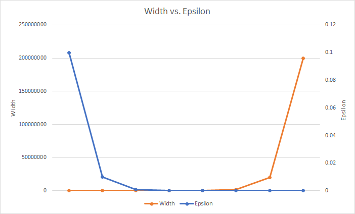
Increasing the width w of the array gives you a smaller error tolerance for overcounting the frequency of an item due to the reduced likelihood of a hash collision within the same hash function within the row. Remember that the width is defined as w = ceil(2/ϵ) so as your tolerance for error (ϵ) decreases, the value of w increases to achieve that. The larger width for the array gives you an increased space complexity that will quickly bring costly space requirements.
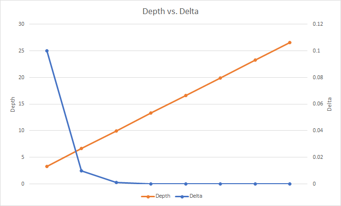
Increasing the depth d of the sketch gives you a higher chance of being within the error tolerance because you now have more pairwise-independent hash functions generating the index for the increment, thus a smaller chance of collisions having increased all counts for any given item. The depth is defined as d = ceil(log2𝛿-1), which may be easier to understand if we show the negative exponent as d = ceil(log21/𝛿) instead. Now it looks similar to 2/ϵ for the width w above, except we're calculating log21/𝛿 instead and it gives us a nice linear increase in depth vs. our probability to be in tolerance.
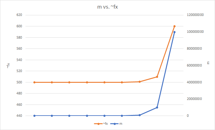
The last thing in our control is the number of items in the Sketch, m. Remember earlier that we said Pr(~fx <= fx + ϵm) <= 1 - 𝛿 and I drew attention to how the estimated frequency (~fx) that the CMS will tell us is less than or equal to the true frequency (fx) plus the error tolerance multiplied by the number if items in the data stream (ϵm) with a certain probability (1 - 𝛿)? Well, as we add more items to the CMS, we increase the chance that hash collisions will again start to increase counts for other items. A CMS is somewhat resistant to this as we are storing multiple counts for each item, but it is still a factor as we increase the number of items. It's also worth pointing out that m is the number of unique items and not the number of increment operations. If we have 1 item with a count of 1,000,000, then m = 1, but if we have 1,000,000 items with a count of 1, then m = 1,000,000. The inaccuracy of ~fx is then directly related to m and is shown here with:
ϵ = 0.000001
fx = 500
Low Cost
As we already have some quite nice Redis Servers it's not too difficult to find the capacity to add the above Count-Min Sketch. Even if you don't have an existing Redis Server, looking at our VPS provider, DigitalOcean, you could spin one up that's capable of handling the largest requirements above for only $48/mo.
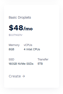
If you cut the space requirements down and only go as far as a 32bit integer for the counts and still go for the biggest Count-Min Sketch we looked at above, it brings the price down to just $24/mo!
The link above gets you $100 in credit when you sign up so you could create the larger server and test it out for 2 months without spending a penny too. As we start to implement more awesome features at Report URI, I plan to keep blogging about them and there's at least one more probabilistic data structure we're looking at implementing soon, so stay tuned, but that leads me on to my final point.
Limitations of Count-Min Sketch
Doing frequency analysis on events like I've shown above with a CMS is amazing and with such low overheads, it's a very attractive solution. We can take any inbound report and check to see if we've seen that report before, let's say it has a count close to 0, or if it's a very rare report, because it has a low count. We can also see if we've seen a report tens of millions of times before, which is also very useful to know. Doing that without touching the database, without storing all historic data and with only a few GBs of RAM is awesome. There is something that a CMS can't tell us though; "What are our top 10 most frequent reports?"
The data is in the CMS, because the count of all reports is in the CMS, but unless you know what your top 10 reports are, you can't query out the count for the top 10 reports... See how that's kind of a problem?! We could even search for the 10 largest counts in the CMS, but that wouldn't tell us which reports they were for! Thankfully, there are a couple of solutions to this problem.
The final probabilistic data structure I'm going to be looking at is Top K, which allows you to determine the Top K, or in my example the Top 10, most frequent items in your data. It differs from CMS in it's operation and structure, but allows us to ask the question "What are our top k most frequent reports?" instead of "How many times have we seen this report?", which is another very important question to answer and something I'll be covering in detail soon!